
Clean Your Data Fast Deleting Duplicates in Excel
Before we jump into the different ways to delete duplicates in Excel, it’s worth taking a moment to understand why this is such a critical skill. Dealing with duplicate data isn't just a minor spreadsheet headache; it's a silent killer for your business operations. It inflates your lead counts, completely skews your marketing analytics, and wastes a ton of resources on sales efforts that go nowhere.
The Hidden Costs of Duplicate Data
Let's paint a picture. Your marketing team just wrapped up three different ad campaigns and pulled all the leads into a single Excel sheet. At first glance, that 5,000-entry list looks amazing. But then you start digging in and realize the same contact information is popping up over and over again, bloating your actual lead count by a solid 20%. This is an incredibly common scenario, and it kicks off a domino effect of expensive problems.
This flowchart really brings home the branching impact that data accuracy—or a lack thereof—has on your business.
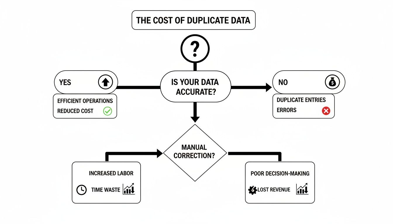
The message here is crystal clear: messy, inaccurate data leads directly to financial and operational losses. On the flip side, clean data is what drives real growth and efficiency.
Why Data Cleaning Is a High-ROI Activity
When you don't take the time to remove duplicates, you're not just looking at a messy file. You're actively undermining your business intelligence and making your teams less efficient. The consequences are real and they hit your bottom line:
- Wasted Marketing Spend: You end up paying to acquire the very same lead multiple times from different sources.
- Skewed Analytics: Those inflated numbers lead to poor strategic decisions because you're working with flawed data.
- Damaged Brand Reputation: Nothing looks more unprofessional than contacting the same prospect repeatedly. It's a fast track to getting unsubscribes and complaints.
- Inefficient Sales Teams: Your sales reps waste precious time chasing the same lead, completely unaware that their colleague is already on it.
This productivity drain is no joke. One recent survey revealed that 68% of users in marketing and sales spend over five hours every single week just cleaning duplicate data out of their spreadsheets. In a typical dataset of 10,000 leads, this kind of duplication can easily inflate the true numbers by 15-25%, leading to completely misguided ad targeting.
This isn't just about tidying up a list; it's about reclaiming lost time and ensuring every dollar spent on marketing and sales is based on accurate, reliable information.
Understanding these costs completely reframes the task of deleting duplicates. It stops being a tedious chore and becomes a critical business process. This really highlights the importance of not just removing them once, but also adopting ongoing efforts for improving overall data quality. To learn more about building a solid foundation, check out our guide on data management best practices.
Your Quickest Fix: The Remove Duplicates Tool
When you need to get rid of duplicate entries in Excel—and you need it done now—the built-in Remove Duplicates feature is your best friend. This is the tool I turn to for a fast, permanent cleanup. It's perfect when you don't need to keep the original data and just want a clean list, fast.
Picture this: you've just exported a fresh lead list from your CRM or a webinar platform. You can already see there are multiple entries for the same person, maybe because they registered with the same email twice. This is exactly what the tool was made for. You can have that list cleaned up in less than a minute.
Getting the Tool to Work
First, you need to tell Excel what data to look at. The easiest way is to click any single cell inside your data table. Excel is pretty smart and usually figures out the entire range on its own.
But for a safer, more precise approach, I always recommend manually highlighting the entire range yourself, headers and all.
Once your data is selected, head over to the Data tab on the ribbon. You'll spot the Remove Duplicates button in the "Data Tools" section. Clicking it brings up a small but crucial dialog box.
Pro Tip: Seriously, always work on a copy of your data. The Remove Duplicates tool permanently deletes rows. Once you save and close that file, there’s no easy undo button. Make a backup of your sheet before you start.
Choosing Your Columns Wisely
This is where the magic happens, and it's the most critical step. The dialog box shows you a list of all the columns in your selected data. By default, Excel checks every single one.
Here’s what that means:
- Checking all columns tells Excel to delete a row only if it’s a 100% carbon copy of another row across every single column.
- Checking specific columns tells Excel to delete rows that have duplicate values only in those specific columns you've picked, ignoring everything else.
Let's use a real-world sales list as an example. You might have the same contact, "Jane Doe" with the email "jane.doe@email.com," listed twice. But one entry has an "Engagement Date" of May 5th, while the other shows June 12th. If you leave all the columns checked, Excel won’t see this as a duplicate because the dates are different.
To get a truly clean lead list, you'd unselect all columns and then check only the 'Email' column. An email address is almost always a unique identifier for a person.
Click 'OK', and Excel will instantly scan your list, keep the very first instance of "jane.doe@email.com" it finds, and permanently delete any others. A little confirmation message will pop up, telling you exactly how many duplicates it zapped, leaving you with a perfectly clean list.
Visually Spot Duplicates With Conditional Formatting
Sometimes, just nuking duplicate rows from orbit isn't the right call. You might need to see them first, understand the context, or figure out why they're there before taking action.
This is where Conditional Formatting becomes your best friend. It’s a fantastic auditing tool that lets you highlight duplicates instead of deleting them, giving you full control over the process. It's a non-destructive approach, meaning your original data stays completely intact.

Let's say you're a marketer merging a new list of leads from a recent campaign into your master database. If you just delete rows with duplicate emails, you might accidentally throw away valuable new information in other columns. By highlighting duplicates in the 'Email' column instead, you can quickly see which new leads are already in your system and decide how to merge their data thoughtfully.
How to Highlight Duplicate Values
Applying this rule is incredibly straightforward and gives you an immediate visual map of your data. It's the perfect first step in any data-cleaning project, especially since you can undo it with a single click.
Here’s how to get it done:
- Select your data range. Just click and drag to highlight the entire column you want to check, like 'Email Address' or 'Phone Number'.
- Head to the Home tab. This is where all the formatting magic happens.
- Find the rule. Click on Conditional Formatting > Highlight Cells Rules > Duplicate Values.
- Pick your color. A small dialog box will pop up. You can leave the default "Duplicate" selected and choose a formatting style from the dropdown menu, like the classic "Light Red Fill with Dark Red Text." Click OK.
Instantly, every cell in your selected range that has a duplicate will light up. This visual feedback is super powerful for getting a quick read on the scale of your duplicate problem.
This method is my personal go-to for an initial data audit. It doesn't change a single thing in your spreadsheet; it just gives you the intel you need to make an informed decision. You get to see the problem before you commit to a solution.
The Strategic Value of Highlighting
The need for this kind of visual check is more common than you might think. A recent study found that a staggering 82% of spreadsheets in major markets contain duplicates, which can skew analytics by up to 30%. Using Conditional Formatting—a feature that's been in Excel since Office 2003—is your fastest first line of defense against this issue. You can dig into these data quality findings in the full Hermes BI report.
This approach empowers you to investigate why the duplicates exist in the first place. Are they simple typos or data entry errors? Or do they represent multiple interactions with the same customer? Answering that question is the key to maintaining a clean, meaningful dataset.
Once the duplicates are highlighted, you can easily filter by color to group them all together for closer inspection or manual cleanup. It puts you firmly in the driver's seat.
When the simple "Remove Duplicates" button just doesn't cut it, it's time to bring out Excel's heavy hitters. For complex data, recurring cleanup tasks, or situations where you absolutely can't risk altering your original dataset, there are more powerful and flexible ways to handle duplicates.
These advanced methods don't permanently delete rows. Instead, they create a new, clean output, leaving your original data completely untouched. This is how the pros handle serious data cleaning—it’s non-destructive, repeatable, and gives you far more control.

Create Dynamic Lists With the UNIQUE Function
If you're using Microsoft 365 or a recent version of Excel, the UNIQUE function is an absolute game-changer. It lets you generate a clean, de-duplicated list from a source range with one simple formula.
The best part? It's dynamic. When you add or change data in your original table, the unique list updates automatically. No re-running anything.
Let's say you have customer orders filling up columns A through C, from row 2 to 100. To create a brand new, de-duplicated table somewhere else on your sheet, you just type this:
=UNIQUE(A2:C100)
That's it. Excel instantly "spills" a new table containing only the unique rows from your original data. This is perfect for building summary reports or dashboards without ever messing with your raw numbers.
Flag Duplicates Using the COUNTIF Formula
An older but still incredibly reliable trick is using the COUNTIF function. This approach doesn't actually remove anything. Instead, it "flags" duplicates by telling you how many times each value appears, giving you a chance to review them.
You can set up a "helper column" next to your data. In that column, you'll use a formula to check how many times a specific value (like an email in cell B2) shows up in the entire column. The formula looks like this:
=COUNTIF(B:B, B2)>1
This will pop up as TRUE for any row that's a duplicate and FALSE for the first time a value appears. From there, you can just filter your data to show only the TRUE values and decide what to do with them. It’s a great way to be methodical and careful.
This formula-based approach gives you a reviewable trail. Unlike the "Remove Duplicates" tool which is a one-and-done action, flagging with COUNTIF lets you analyze the duplicates before committing to deletion.
Automate Data Cleaning With Power Query
For the ultimate in power and automation, nothing in Excel beats Power Query. If you find yourself regularly cleaning up messy data exported from a CRM, ad platform, or database, this is your new best friend.
Power Query (also called Get & Transform Data) lets you build a repeatable, automated workflow for cleaning your data. Here’s the gist of it:
- Load Your Data: First, you pull your table into the Power Query Editor.
- Remove Duplicates: Inside the editor, there's a simple 'Remove Duplicates' button, just like the one in the main Excel ribbon.
- Add More Steps: This is where the magic happens. You can add other cleaning steps, like trimming extra spaces, changing text to lowercase, or splitting columns.
- Load to Your Sheet: Once you're done, you load the clean, transformed data back into a new Excel sheet.
The real power move? That query can be refreshed with a single click. If your original source data changes, just right-click your new table and hit "Refresh." Power Query re-runs all your cleaning steps automatically. For those looking to take their data skills to the next level, understanding how tools like Power Query are a stepping stone to enhancing Excel with Power BI can open up even more powerful reporting capabilities.
Comparing Advanced Deduplication Techniques
When deciding between these methods, it helps to see how they stack up. The right choice depends on whether you need a quick, one-off list or a fully automated, repeatable cleaning process.
| Feature | Remove Duplicates Tool | UNIQUE Function | Power Query |
|---|---|---|---|
| Original Data | Alters it directly | Preserves it; creates a new list | Preserves it; creates a new, refreshable table |
| How it Updates | Manual; must re-run | Dynamic; updates automatically when source changes | Refreshable; updates on demand with one click |
| Ease of Use | Very simple | Simple for single-column, moderate for multi-column | Steeper learning curve, but extremely powerful |
| Best For | Quick, one-time cleanups | Creating dynamic summary lists or dashboards | Automating recurring data cleaning from external sources (CRM, DBs) |
| Additional Cleaning | None | Limited; can be combined with other formulas | Extensive; includes trimming, case changes, splitting, merging, etc. |
Ultimately, while the built-in tool is great for a quick fix, learning to use dynamic formulas like UNIQUE and the automation powerhouse of Power Query will save you countless hours and prevent costly errors in the long run.
How to Handle Tricky and Hidden Duplicates
Ever run the Remove Duplicates tool, only for it to proudly announce "0 duplicate values found"… even when you can see them right there in the sheet? It’s one of the most frustrating parts of cleaning data.
Don't worry, the tool isn't broken. It's just incredibly literal.
To Excel, "Jane Doe " (with an extra space at the end) and "jane doe" (in lowercase) are completely different things. Standard tools miss these hidden variations every single time because they demand a perfect, character-for-character match. This is where you have to get a bit more creative and clean your data before you try to dedupe it.
The Power of Helper Columns
The absolute best way to tackle these invisible inconsistencies is with a "helper column." This is just a temporary column you add next to your original data. In this new column, you’ll use a couple of simple formulas to standardize everything, creating a clean version of your data that Excel can finally work with.
The two formulas you need to know are TRIM and LOWER.
- The
TRIMFunction: This little gem zaps any extra spaces from the beginning or end of a cell's text. That sneaky space after "Jane Doe " will vanish instantly. - The
LOWERFunction: This one converts all text to lowercase, getting rid of any capitalization differences between "Jane" and "jane."
You can even nest them together into one super-formula. If your messy names are in column A, you’d create your helper column (let's say, column B) and enter this formula in cell B2: =LOWER(TRIM(A2)). Drag that formula all the way down your list, and you'll have a perfectly standardized set of names to run the Remove Duplicates tool on.
By creating a clean helper column, you're not just finding more duplicates; you're fixing the root cause of many common data entry errors. It's a foundational skill for anyone serious about accurate data management.
Creating a Unique ID from Multiple Columns
What about when a duplicate isn't just based on one column? Imagine a contact list where you have "John Smith" in row 10 and another "John Smith" in row 150. They could be the same person, or they could just share a common name. To be sure, you often need to check for duplicates based on a combination of data—like First Name, Last Name, and Company.
While the Remove Duplicates tool lets you select multiple columns, another slick method is to create your own unique ID by combining them. This process is called concatenation.
Let's say First Name is in column A and Last Name is in column B. In a new helper column, you can use the formula =A2&B2. This smashes the values together, creating a unique string like "JohnSmith". Once you drag this formula down, you can run Remove Duplicates on this new helper column to find entries that are true duplicates across both fields.
This technique is a lifesaver when you're merging lead lists from different sources, like a CRM export and a webinar signup sheet, where formatting is almost never consistent. For a deeper dive into preventing these issues in the first place, our guide on common data entry errors has some great strategies.
By mastering these simple functions, you’ll elevate your data cleaning skills from basic to pro level.
Beyond Excel: Putting Your Data Cleaning on Autopilot
Okay, so you've gotten pretty good at wrestling duplicates into submission with Excel's tools. That's a solid skill to have. But let's be honest, for any business that's trying to grow, a bigger question starts to loom: how do we stop this mess from happening in the first place?
Every hour you spend cleaning up a CSV export is an hour you're not spending on strategy, talking to clients, or actually closing a deal. Manual data cleaning is a classic growth bottleneck.

This is where you graduate to automated data integration. Instead of the whole download-open-clean-upload routine, you can use tools that sync clean, deduplicated leads directly from your sources (like Facebook Lead Ads) right into your systems. The entire cleanup process just… disappears.
The Strategic Shift to Prevention
Think of this as a strategic upgrade, not a replacement for your Excel knowledge. Knowing how to fix messy data is invaluable, but preventing the mess from ever reaching you is a massive competitive advantage.
When you take a proactive approach, you save a ton of time. More importantly, it means your sales and marketing teams can jump on pristine, accurate leads the second they come in.
Microsoft's own support data shows that 75% of PivotTable users are constantly fighting duplicates. These rogue entries can inflate your counts by an average of 20%, which completely throws off your ROI calculations. We've seen businesses waste hours every week on this.
On the flip side, tools that automatically filter duplicates at the source can boost lead response rates by as much as 35% just by delivering clean data instantly. You can dig into some of these findings on duplicate data from Microsoft yourself.
The best way to solve the problem of deleting duplicates in Excel is to avoid having them in your spreadsheets to begin with. Automation is the key to achieving this level of data hygiene.
By making this change, you're breaking the reactive cycle of constant cleanup. This allows your business to scale operations, act on opportunities faster, and finally trust the data that's driving your decisions.
If you're curious how this works in practice, you might want to check out our article on what is workflow automation and see how it can completely transform your lead management process.
Got Questions About Removing Duplicates?
Even with the best tools, you're bound to run into some tricky situations when cleaning up your data. This is where people usually get stuck. Let's tackle some of the most common questions that pop up when you're trying to get rid of duplicates in Excel.
Think of this as your quick-reference guide for those "what if" scenarios that can derail an otherwise smooth data-cleaning session.
How Do I Keep Just the First Record?
This is a big one. You want to delete the copies, not the original. The good news is that Excel’s built-in Remove Duplicates feature is designed to do exactly this.
When the tool finds a set of duplicate rows (based on the columns you told it to check), it automatically keeps the very first record it comes across in your list. It then zaps all the other matching rows that appear after it. This is the default setting, so you don't need to do anything special to make it happen. It just works.
Can I Find Duplicates Across Two Different Sheets?
Absolutely, but you'll need to get a bit more creative than the basic tools. This scenario is perfect for when you're checking a new list of leads against your master database.
The easiest way to handle this is with a COUNTIF formula combined with Conditional Formatting. Let's say you want to highlight cells in Sheet1 that also show up in Sheet2. Just set up a new Conditional Formatting rule with this formula:
=COUNTIF(Sheet2!A:A, A1)>0
This little formula checks every cell in column A of your current sheet (Sheet1) and lights it up if it finds a match anywhere in column A of your other sheet (Sheet2).
I find this method incredibly handy for visually checking new data imports before I merge them. It's a simple way to stop yourself from adding even more duplicates into your main database.
Why Isn't Remove Duplicates Working?
This is a classic. You can see the duplicates, but Excel insists there aren't any. Almost every time, this is because of tiny inconsistencies that are invisible to us but glaring to a computer. Excel needs a perfect, character-for-character match to flag a duplicate.
The usual suspects are:
- Hidden extra spaces lurking at the beginning or end of a cell.
- Inconsistent capitalization, like "Acme Inc." vs. "acme inc.".
Here’s the fix: create a temporary "helper column" next to your messy data. Use the TRIM and LOWER functions to standardize everything. A formula like =LOWER(TRIM(A2)) will clean up the text in cell A2 by removing extra spaces and making it all lowercase.
Drag that formula down your entire column, then run the Remove Duplicates tool on your new, clean helper column. Now it will find all those matches it missed before.
Stop wasting time on manual CSV downloads and start acting on leads instantly. LeadSavvy Pro automates your entire Facebook lead capture process, syncing clean, de-duplicated leads directly to your Google Sheet or CRM. Get started for free today.